Practical 2 - Experimental design

Sampling data and more

Author

Dr William Kay

Published

October 28, 2025

Learning Outcomes (LOs)

Here’s what you should know and be able to do after completing this practical:

LO1: Explain different sampling methods
LO2: Write code to perform different sampling methods
LO3: Simulate data, including from different distributions
LO4: Run a basic loop
LO5: Set a “seed” and explain what it does
LO6: Explain how increased sample size affects estimates (of things like mean values)
LO7: Subset data using subset() and indexing
LO8: Explain the importance of replication

TUTORIAL

Simulating data and distributions

In this script will we be working with entirely simulated data. In other scripts, we will use more real data, but to exemplify experimental design concepts, it’s actually I think more helpful to work with simulated data.

Let’s imagine a population that consists of 100,000 individuals.

In this first example, we are going to simulate the heights of 100,000 people.

Across the world, people differ in their heights considerably, but on average if you look across all adults, regardless of sex or gender, it’s reasonable to consider a typical mean height of 170 cm with a standard deviation of 10 cm. For examples, see: https://en.wikipedia.org/wiki/Average_human_height_by_country

So, let’s simulate a single variable, which is normally distributed and has a mean of 170 and a SD of 10.

I’m calling this variable popHeights (population heights):

popHeights <- rnorm(100000, 170, 10)

This variable has been created using the rnorm() function, which generates random numbers from a normal distribution

If you want to see how the rnorm function works (or any function for that matter), type “?” followed by the function name:

?rnorm

We saw rnorm() in the first script (Practical 1 - Basics of R) but as a reminder:

The rnorm() function has three arguments: n, mean, and sd

n = the number of observations you want to simulate
mean = this is the mean value of the normal distribution you want to simulate from
sd = this is the sd of the distribution

If we wanted to, we could plot a quick histogram of the population heights, to take a look:

hist(popHeights)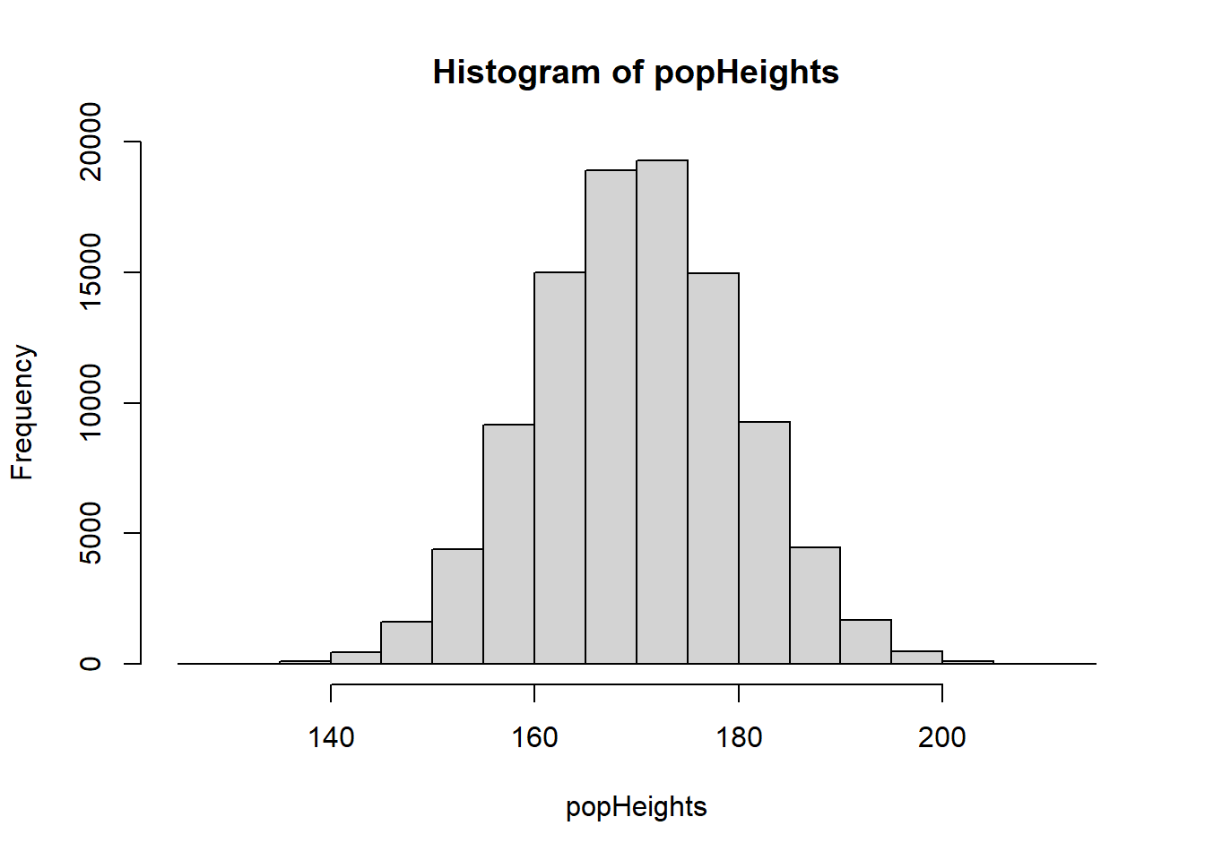

Remember that in most scientific experiments, we wouldn’t collect data from the entire population.

We would instead collect a sample. Let’s look at how to do this:

Suppose we want to measure the heights of a sample of 50 people from our population.

We can use the sample() function. We’ll store the sample of heights in a new object called sHeights:

sHeights <- sample(popHeights, 50, replace = FALSE)

Importantly, in the above function I set replace = FALSE. This is to tell R that once an individual has been selected, they cannot be selected again. This is known as sampling without replacement and is typical for real world surveys, because you may not want to sample the same person’s height twice.

If I were to set replace = TRUE, this would simulate sampling with replacement: after selecting an individual, that person is returned to the population and could be chosen again.

Scientists sometimes do this in simulations to see how results might vary if we repeated an experiment.

You don’t need to worry about this for now — just know that it exists.

Lets look at our sample distribution:

hist(sHeights)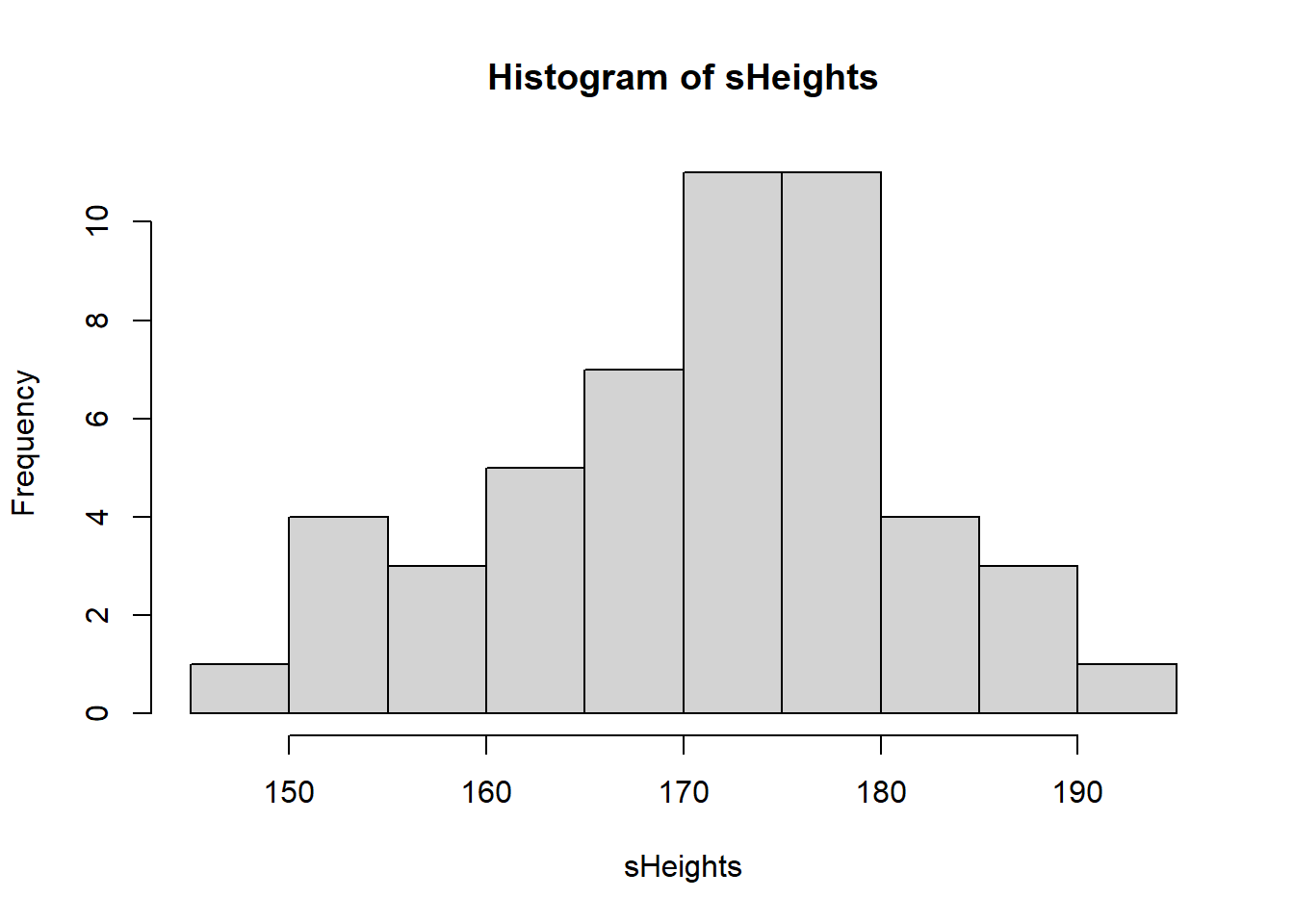

We could, if we wanted to, calculate the mean of our sample:

mean(sHeights)

[1] 171.263

We will explore sample distributions in more detail later. For now, let’s simulate a slightly more realistic scenario - one where we don’t just collect data on 1 variable, but on a few different variables.

Let’s imagine a population of 100,000 humans who all have different heights, weights, ages, etc.:

population <- data.frame(
  height = rnorm(100000, 170, 10),
  weight = rnorm(100000, 65, 10),
  age = rnorm(100000, 40, 15),
  systolic_bp = rnorm(100000, 120, 15), 
  diastolic_bp = rnorm(100000, 80, 10), 
  cholesterol = rnorm(100000, 5, 1), 
  gender = sample(c("Male", "Female", "Other"), 100000, replace = TRUE, prob = c(0.49, 0.49, 0.02)),
  ethnicity = sample(c("White", "Black", "Asian", "Other"), 100000, replace = TRUE, prob = c(0.3, 0.3, 0.3, 0.1)), 
  university = sample(LETTERS[1:10], 100000, replace = TRUE, prob = rep(0.1, 10))
)

This simulation should take less than 1 second. R can handle very large datasets very quickly!

Let’s make sure we tell R that the gender, ethnicity, and university variables are all categorical (factors):

population$gender <- as.factor(population$gender)

population$ethnicity <- as.factor(population$ethnicity)

population$university <- as.factor(population$university)

For gender, we’ve simulated a population where 49% of people are male, 49% are female, and 2% identify as another gender (e.g., non-binary, transgender, etc.).

For ethnicity, we’ve simulated a scenario where 30% of people are White, 30% are Black, 30% are Asian, and 10% belong to other ethnic groups.

NOTE: These gender and ethnicity proportions are entirely hypothetical and are not intended to reflect real-world population data.

We’ve also simulated these people all attending one of 10 different universities.

Let’s take a look at the first few rows of the dataset we just created:

head(population)

    height   weight       age systolic_bp diastolic_bp cholesterol gender
1 181.8917 65.95659 54.043762   136.72015     76.27696    6.751264   Male
2 152.3525 69.73649 41.885823   121.98966     91.00437    4.852896   Male
3 161.9172 51.98096 28.842420    89.06611     86.36814    4.673087   Male
4 175.1414 72.10186  9.956617   110.30854     77.83300    6.643298   Male
5 165.9646 61.66644 27.424063   110.96473     73.16775    5.290861   Male
6 184.8499 64.55127 14.819444   124.52521     80.13347    3.699011   Male
  ethnicity university
1     Other          F
2     Asian          F
3     White          G
4     White          I
5     Black          D
6     Black          I

Now we can start looking at some of the possible sampling strategies we might use to sample from this population.

Random sampling

Pick 30 individuals at random from the entire population.

First we create an object called rowNums. In this we store 30 random numbers from 1:100000:

rowNums <- sample(1:100000, 30, replace = F)

Then, we use that to select which rows to choose when performing indexing on our population:

random_sample <- population[rowNums, ]

Let’s look at the first few of these randomly sampled individuals:

head(random_sample)

        height   weight      age systolic_bp diastolic_bp cholesterol gender
4653  169.7799 73.37108 62.72067    104.5133     64.65091    4.631331 Female
11246 184.7911 66.92005 59.24338    119.6797     81.44419    6.266655 Female
34408 180.0082 57.18565 44.89194    113.0768     85.72993    6.560816   Male
17171 172.0403 77.29059 44.31937    131.6149     70.51090    4.887556   Male
95866 164.9999 65.87086 45.13674    100.5497     86.16386    4.251617   Male
42490 185.3999 58.80658 57.34801    112.5643     77.93042    7.105784  Other
      ethnicity university
4653      Black          H
11246     Other          B
34408     Asian          E
17171     Black          J
95866     White          D
42490     Asian          J

Note that the first column that you see represents the original row numbers within the population

Systematic sampling

Let’s now choose every 100th individual within the population. Let’s start by creating a sequence which takes every 100th individual starting from individual number 1:

seq1 <- seq(1, 100000, 100)

Then, we use this seq1 in our indexing:

systematic_sample <- population[seq1, ]

Let’s look at the first few rows of these:

head(systematic_sample)

      height   weight       age systolic_bp diastolic_bp cholesterol gender
1   181.8917 65.95659 54.043762    136.7201     76.27696    6.751264   Male
101 153.8822 73.98783 46.436233    113.2102     77.79679    5.047658   Male
201 152.9155 69.85994  3.292137    132.2375     77.24115    5.789151   Male
301 157.7660 59.62766 30.774110    113.9843     81.75128    4.588415   Male
401 174.3276 75.95124 42.307131    113.4292     74.93412    5.390191 Female
501 165.3558 64.54569 -6.853938    108.5050     72.25534    6.938712 Female
    ethnicity university
1       Other          F
101     Asian          C
201     Black          J
301     Asian          C
401     Asian          I
501     Other          I

Stratified random sampling

In stratified random sampling we want to take a sample that proportionally represents the population.

Let’s look at taking a stratified random sample according to gender.

Before we take a sample, we need to work out how many individuals we have of each gender. The table() function is good for this:

table(population$gender)


Female   Male  Other 
 49051  48944   2005

So this is how many individuals we have of each gender. But what about as a proportion?

For this we can apply the prop.table() function to this table:

prop.table(table(population$gender))


 Female    Male   Other 
0.49051 0.48944 0.02005

So we have 48.634% female, 49.306% male, and 2.06% other.

To keep things simple, let’s round these numbers to whole percentages: 49%, 49% and 2%.

We can now use those values to perform our stratified random sampling.

Imagine we wanted a sample of 100 individuals in total. To keep our sample proportionally representative of the population, that would mean we have 49 male, 49 female, and 2 other.

Here’s one way to do this. First, create some subsets:

male <- subset(population, gender == "Male")

female <- subset(population, gender == "Female")

other <- subset(population, gender == "Other")

Now, we can randomly sample 49, 49, and 2 individual from these respectively:

sMale <- male[sample(1:nrow(male), 49, replace = FALSE), ]

sFemale <- female[sample(1:nrow(female), 49, replace = FALSE), ]

sOther <- other[sample(1:nrow(other), 2, replace = FALSE), ]

Explanation of the above:

For each gender, we first create a subset of the population.
Then we use sample() to randomly select the desired number of rows.
The 1:nrow(data) part creates a sequence of row numbers that is specific to each dataset so that the sample() function knows which rows to pick from.

We now have our three subsets. We can combine them using rbind(), which stands for “row bind”.

rbind() stacks the datasets on top of each other (adds rows), so all the selected individuals are together in one dataset. This works because all three subsets have the same columns and structure.

stratified_sample <- rbind(sMale, sFemale, sOther)

Let’s have a look at this sample either using head() or View():

head(stratified_sample)

        height   weight      age systolic_bp diastolic_bp cholesterol gender
41026 163.0809 70.69900 23.99529    121.0283     87.63013    4.546431   Male
55159 169.7011 44.96024 81.78328    120.0054     77.30928    5.193442   Male
97107 167.0441 69.72781 31.83209    132.2845     78.10886    5.986965   Male
95298 169.7894 58.40553 39.36326    123.5954     63.41858    5.950757   Male
65343 181.0432 68.40817 37.29478    117.4471     79.47869    4.785539   Male
32980 171.3221 70.93626 26.34709    143.2521     91.34546    3.977288   Male
      ethnicity university
41026     Black          H
55159     White          H
97107     Other          G
95298     White          G
65343     Asian          H
32980     Black          E

View(stratified_sample)

Quota sampling:

We can use a very similar approach to perform quota sampling.

Let’s assume we want data on 5 individuals from each ethnicity.

First, create ethnicity subsets:

Asian <- subset(population, ethnicity == "Asian") 
Black <- subset(population, ethnicity == "Black") 
White <- subset(population, ethnicity == "White") 
Other <- subset(population, ethnicity == "Other")

Now select 5 individuals from each subset:

sAsian <- Asian[sample(1:nrow(Asian), 5, replace = FALSE), ] 
sBlack <- Black[sample(1:nrow(Black), 5, replace = FALSE), ] 
sWhite <- White[sample(1:nrow(White), 5, replace = FALSE), ] 
sOther <- Other[sample(1:nrow(Other), 5, replace = FALSE), ]

And again rbind() them:

quota_sample <- rbind(sAsian, sBlack, sWhite, sOther)

Have a look, this time just print the entire dataset as it’s only small (20 individuals):

quota_sample

        height   weight      age systolic_bp diastolic_bp cholesterol gender
66546 173.6025 65.00084 47.53982    109.6991     93.29653    5.238933 Female
59742 188.7630 53.85722 47.09415    117.3835     73.97170    3.052515   Male
89278 191.3660 55.22209 16.05946    124.1786     86.84495    4.718466   Male
38398 169.1332 62.30335 42.91705    126.4840     83.46747    3.161352 Female
49287 171.4612 68.06520 45.68254    126.2581     63.05222    3.301955 Female
34276 195.7192 61.38782 48.57233    121.3732    102.17456    5.249173   Male
46415 164.5650 66.82846 32.71044    137.0233     88.01298    4.953049 Female
56297 179.5274 71.38645 42.22164    107.8484     90.41166    5.612718 Female
3843  193.7212 61.34739 46.56138    107.6604     73.73065    3.822007 Female
37406 157.2184 49.27461 22.60050    121.9938     61.83209    4.713379   Male
48112 169.0804 62.32836 75.49070    141.8244     96.73715    5.175702   Male
98442 172.1584 71.47122 36.99733    145.7300     63.61692    4.495889   Male
87550 177.0591 55.39918 35.61092    116.5942     76.22142    4.509009   Male
78117 168.9749 74.80501 31.51017    116.2274     85.85864    3.765290   Male
51190 169.1691 80.52377 40.78356    120.7377     75.10947    5.701031 Female
43518 163.3178 67.07632 51.71008    116.4906     67.72671    6.632093 Female
68953 173.7001 73.49131 25.22929    129.7150     84.22430    4.068652 Female
75349 175.6710 64.12274 29.81824    118.2672     95.02906    5.384948   Male
20645 169.8536 58.92705 50.05220    120.7502     69.51482    4.399490 Female
29078 174.2245 77.72705 17.44857    115.0675     77.37110    4.892672   Male
      ethnicity university
66546     Asian          E
59742     Asian          C
89278     Asian          B
38398     Asian          D
49287     Asian          B
34276     Black          H
46415     Black          B
56297     Black          B
3843      Black          F
37406     Black          B
48112     White          A
98442     White          B
87550     White          G
78117     White          H
51190     White          G
43518     Other          I
68953     Other          A
75349     Other          H
20645     Other          I
29078     Other          G

Cluster sampling:

Finally, let’s take a look at cluster sampling.

This is where we might select only a few specific clusters (characteristics), but include all individuals who have those characteristics. For example, let’s imagine we only wanted to look at people who went to three different universities (university A, B, and C):

A <- subset(population, university == "A") 
B <- subset(population, university == "B") 
C <- subset(population, university == "C")

In cluster sampling, we collect data on all individuals from those clusters. So we don’t need to perform any further sampling, we just rbind() the entire three clusters together:

ABC <- rbind(A, B, C)

Now we can have a look at it:

head(ABC)

     height   weight      age systolic_bp diastolic_bp cholesterol gender
25 160.9578 76.54681 29.75255    128.2268     79.00476    5.783385   Male
26 155.6095 53.22573 47.03772    105.5600     79.58648    5.425473 Female
27 180.7766 69.03992 66.54862    117.5942     72.96604    4.005896 Female
36 163.4919 79.29393 22.46824    113.0934     96.06150    4.308785   Male
44 162.7147 69.23167 27.00450    102.5662     80.19901    5.043619 Female
54 174.8940 72.48711 41.74273     95.3446     96.78921    3.311160 Female
   ethnicity university
25     White          A
26     White          A
27     White          A
36     Asian          A
44     White          A
54     Other          A

tail(ABC)

        height   weight       age systolic_bp diastolic_bp cholesterol gender
99927 175.4463 75.44739 42.956506   122.65891     80.68062    5.469707 Female
99929 170.6889 77.88772 45.373440    98.72096     62.88210    5.031693   Male
99934 157.8411 58.80335 50.913249   142.86610     85.94856    7.020991 Female
99969 180.2466 63.48501 34.314829   111.83394     65.75705    4.969786 Female
99976 177.2251 87.76495 38.609772   121.16693     65.15839    4.654630 Female
99985 174.5995 66.53489 -1.957121   120.00469     84.89809    5.008957   Male
      ethnicity university
99927     White          C
99929     Black          C
99934     White          C
99969     Asian          C
99976     White          C
99985     Asian          C

table(ABC$university)


    A     B     C     D     E     F     G     H     I     J 
10064 10205 10135     0     0     0     0     0     0     0

Notice how even though there are no longer any observations in the D-J universities, those categories still exist?

We can remove empty categories by using the droplevels() function:

ABC <- droplevels(ABC)

Now look again:

table(ABC$university)


    A     B     C 
10064 10205 10135

Simulating data from different distributions

So far, whenever we have simulated numerical data, we have used the rnorm() function

This will specifically simulate data from a normal distribution.

Let’s have another quick look at this: let’s simulate 100 normally distributed height observations

heights <- rnorm(n = 100, mean = 170, sd = 10)

We can look at this distribution using hist()

hist(heights)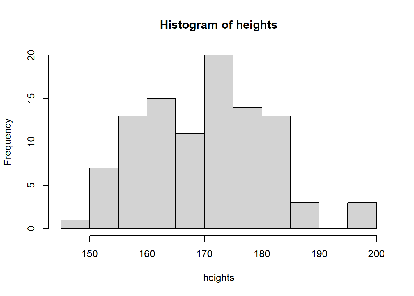

R can simulate data from many different distributions. Let’s look at a few examples.

Poisson Distribution

The Poisson distribution models count data (whole numbers like 0, 1, 2 etc.).

It has a single parameter, lambda, which determines both the mean and the variance.

An obvious biological example of count data are the number of eggs a bird lays.

Here we simulate 100 random numbers from a Poisson distribution with lambda = 2:

pois <- rpois(n = 100, lambda = 2)

Again, we can visualise the simulated data with a histogram:

hist(pois, main = "", xlab = "Number of eggs laid", las = 1)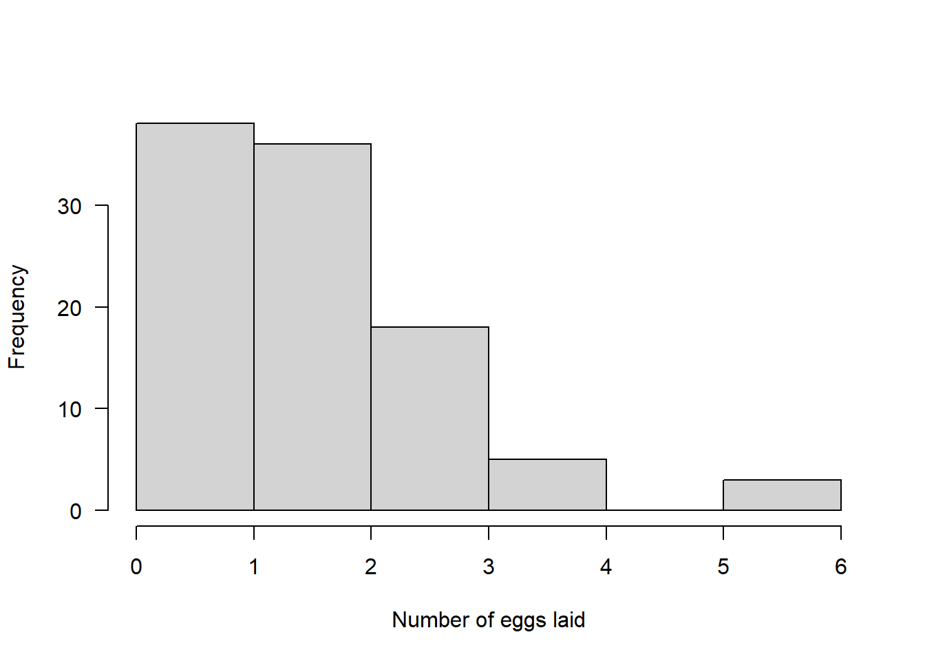

Binomial Distribution

The binomial distribution models data that exists in one of two categories, e.g., success/failure.

Biological example: We have 100 people suffering from pain and we want to test if a drug can reduce it.

rbinom() parameters:

n = number of individuals we are simulating (100 here)
size = number of “trials” per individual (1 if they get the drug once)
prob = probability of success on each trial (probability the drug works)

Example 1: Drug has 50% chance to reduce pain

binom <- rbinom(n = 100, size = 1, prob = 0.5)

hist(binom, main = "", xlab = "0 = Same pain, 1 = Reduced pain", las = 1)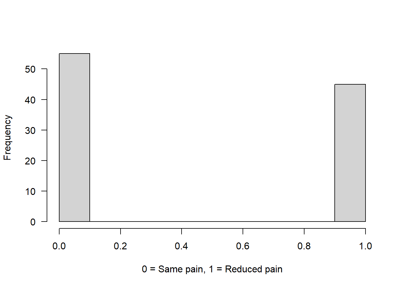

Example 2: Drug has 75% chance to reduce pain

binom2 <- rbinom(n = 100, size = 1, prob = 0.75)

hist(binom2, main = "", xlab = "0 = Same pain, 1 = Reduced pain", las = 1)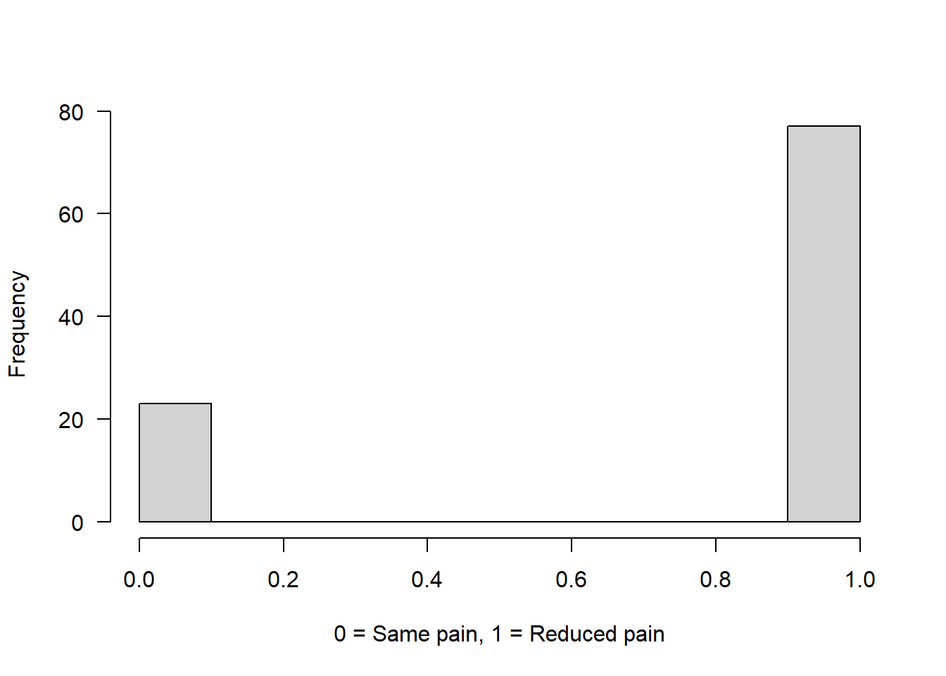

Example 3: Each person gets 2 doses of the drug (size = 2)

The number now represents how many times the drug successfully reduced pain out of two attempts.

Assuming that on both attempts the chance of reducing pain was 75%:

binom3 <- rbinom(n = 100, size = 2, prob = 0.75)

hist(binom3, main = "", xlab = "Number of times pain was reduced (0, 1, 2)", las = 1)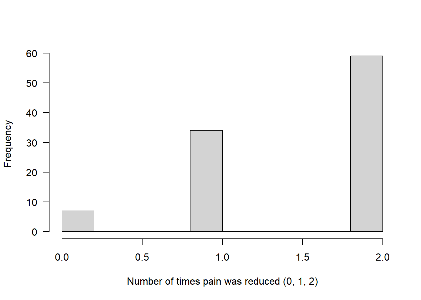

Bimodal distribution

You may remember from the exploring data and graphing lecture, I mentioned that spiders are often sexually dimorphic - females are typically larger than males.

For this you will need to install another package (if that doesn’t work, just skip over this bit):

install.packages("FamilyRank")

library(FamilyRank)

This distribution needs a total sample size, a mean and SD for each of the two peaks (modes) in the distribution, and a probability value which dictates the probability of being in mode 1.

binorm <- rbinorm(n = 200,   # 200 spiders in total 
                  mean1 = 2, # mean for mode 1 (think of male spider diameter in cm) 
                  mean2 = 4, # mean for mode 2 (think of female spider diameter in cm) 
                  sd1 = 0.3, # SD for male spider diameter 
                  sd2 = 0.5, # SD for female spider diameter 
                  p1 = 0.5)  # Probability of being a male spider (50%)

hist(binorm, main = "", las = 1, xlab = "Spider diameter (cm)")

There are many more possible distributions that data can follow, but we will stop here for now!

Just remember (i) that data can follow different distributions - it won’t always be “normal” and (ii) that for many “Parametric” statistical tests, the tests assume your data are normal - so you must check! We will cover this in detail in the next script.

Examining distributions

Let’s have a look at some averages, and variation, of the distributions created above:

Normal

hist(heights) 
abline(v = mean(heights), col = "blue", lwd = 2) 
abline(v = median(heights), col = "red", lwd = 2)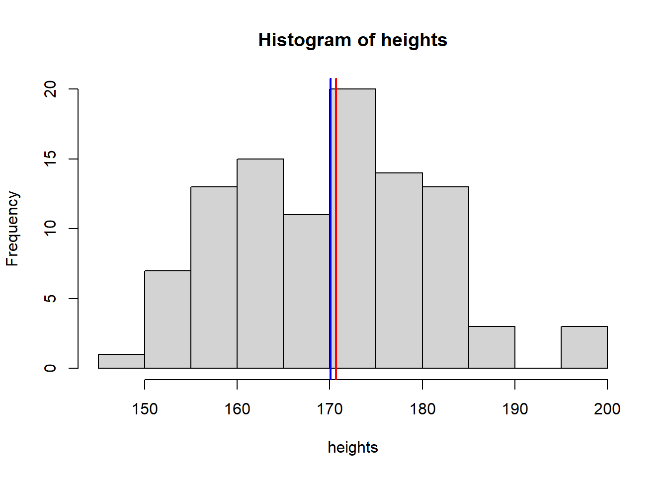

mean(heights)

[1] 170.0839

median(heights)

[1] 170.6889

sd(heights)

[1] 10.73436

Poisson

hist(pois) 
abline(v = mean(pois), col = "blue", lwd = 2) 
abline(v = median(pois), col = "red", lwd = 2)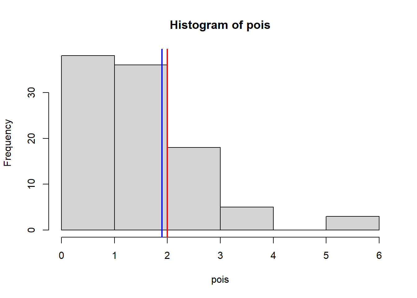

mean(pois) # This should be close to 2

[1] 1.9

var(pois)  # This should be close to 2

[1] 1.606061

Binom

hist(binom) 
abline(v = mean(binom), col = "blue", lwd = 2) 
abline(v = median(binom), col = "red", lwd = 2)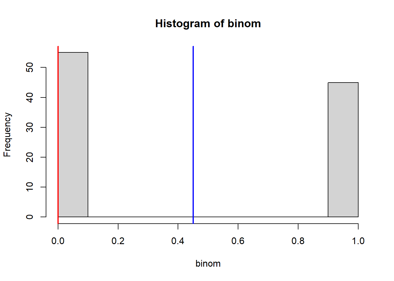

mean(binom)  # This should be close to 50 %

[1] 0.45

table(binom) # This should be close to a 50/50 split!

binom
 0  1 
55 45

Binorm

hist(binorm) 
abline(v = mean(binorm), col = "blue", lwd = 2) 
abline(v = median(binorm), col = "red", lwd = 2) 
mean(binorm) # The mean of a bimodal distribution is not representative of a "typical" or "average" spider! 
sd(binorm)

Hopefully this exemplifies that best representation of the “average” value in a distribution isn’t always the mean!

The importance of sample size

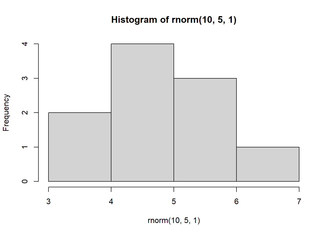
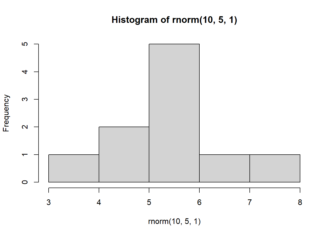
Look at what happens when we create a normal distribution with 10, 100, or 1000 observations:

hist(rnorm(10,5,1))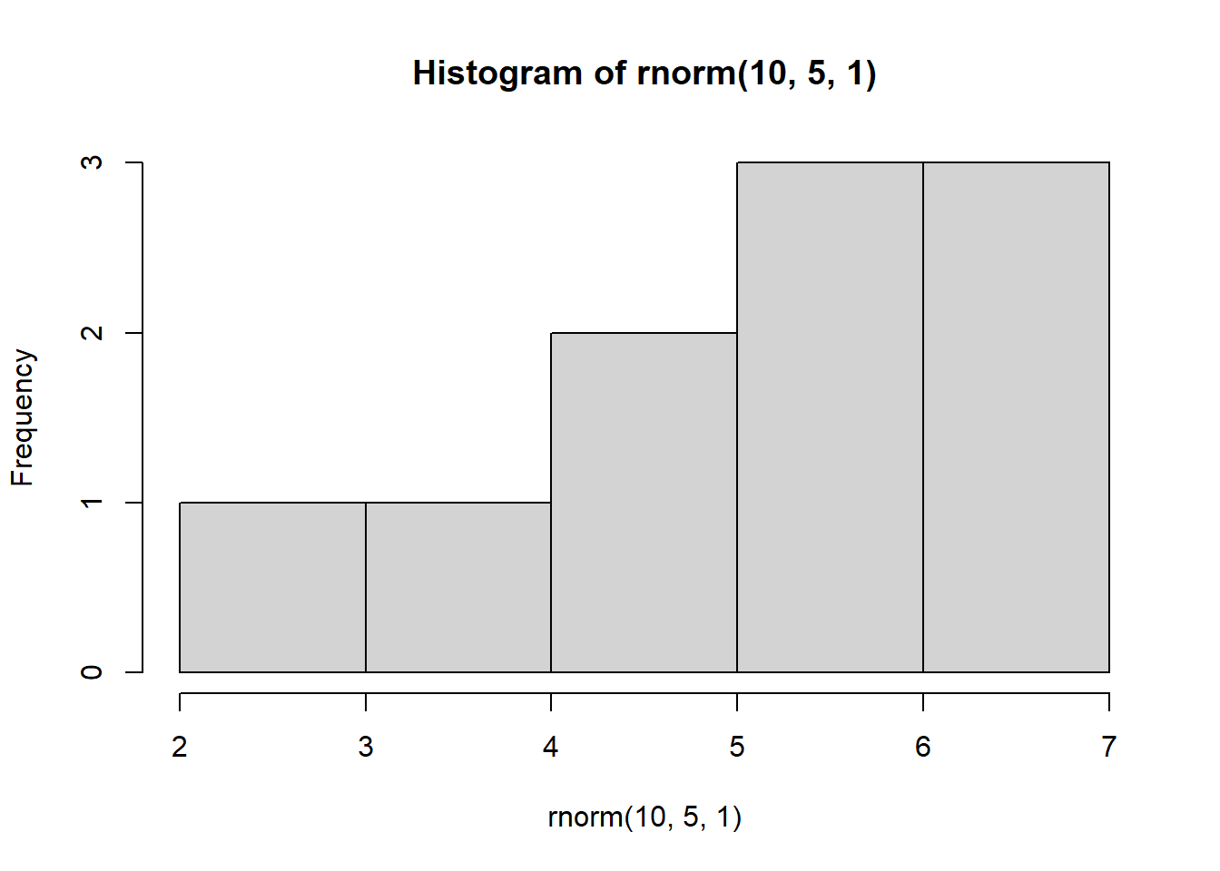

hist(rnorm(100,5,1))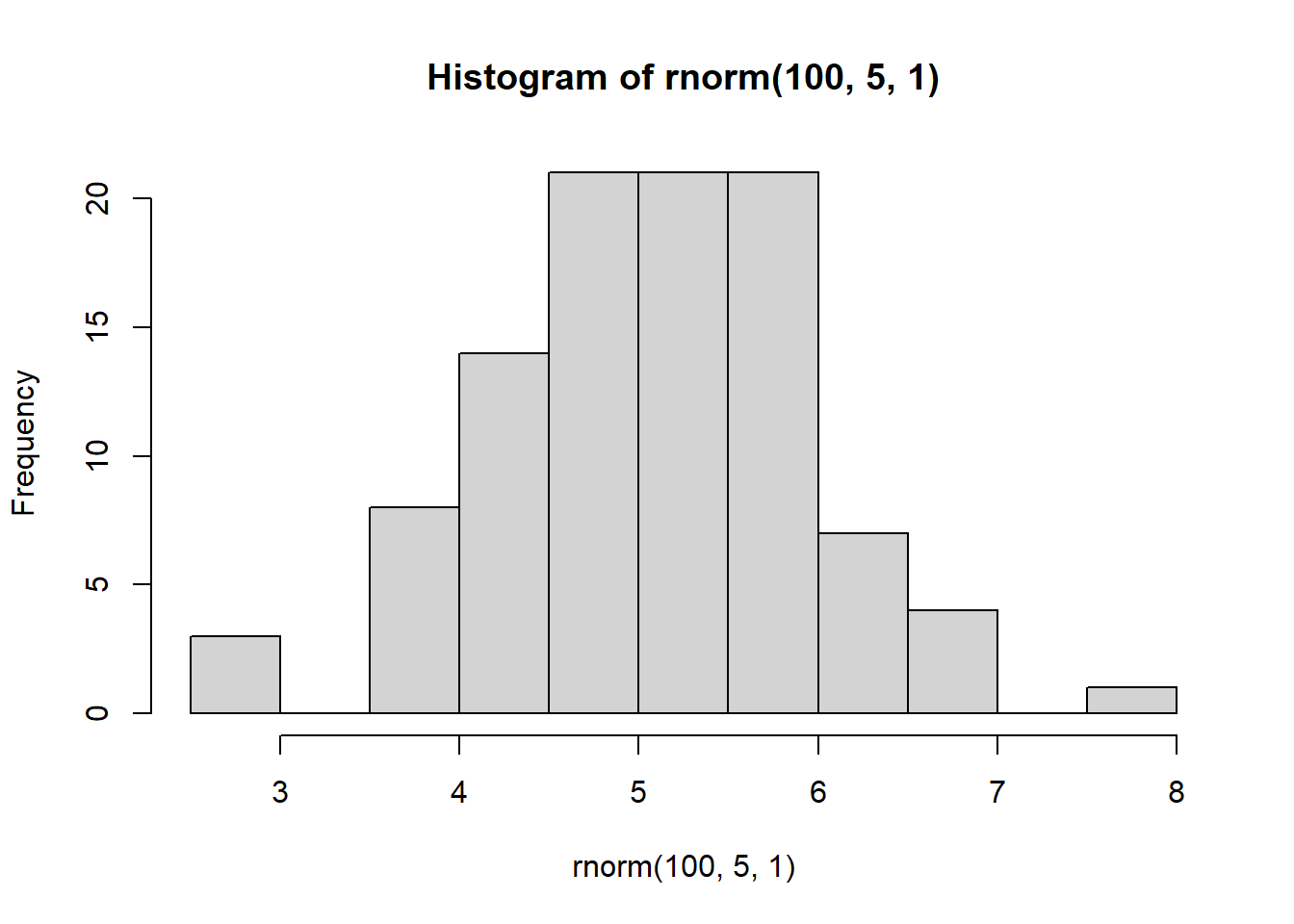

hist(rnorm(1000,5,1))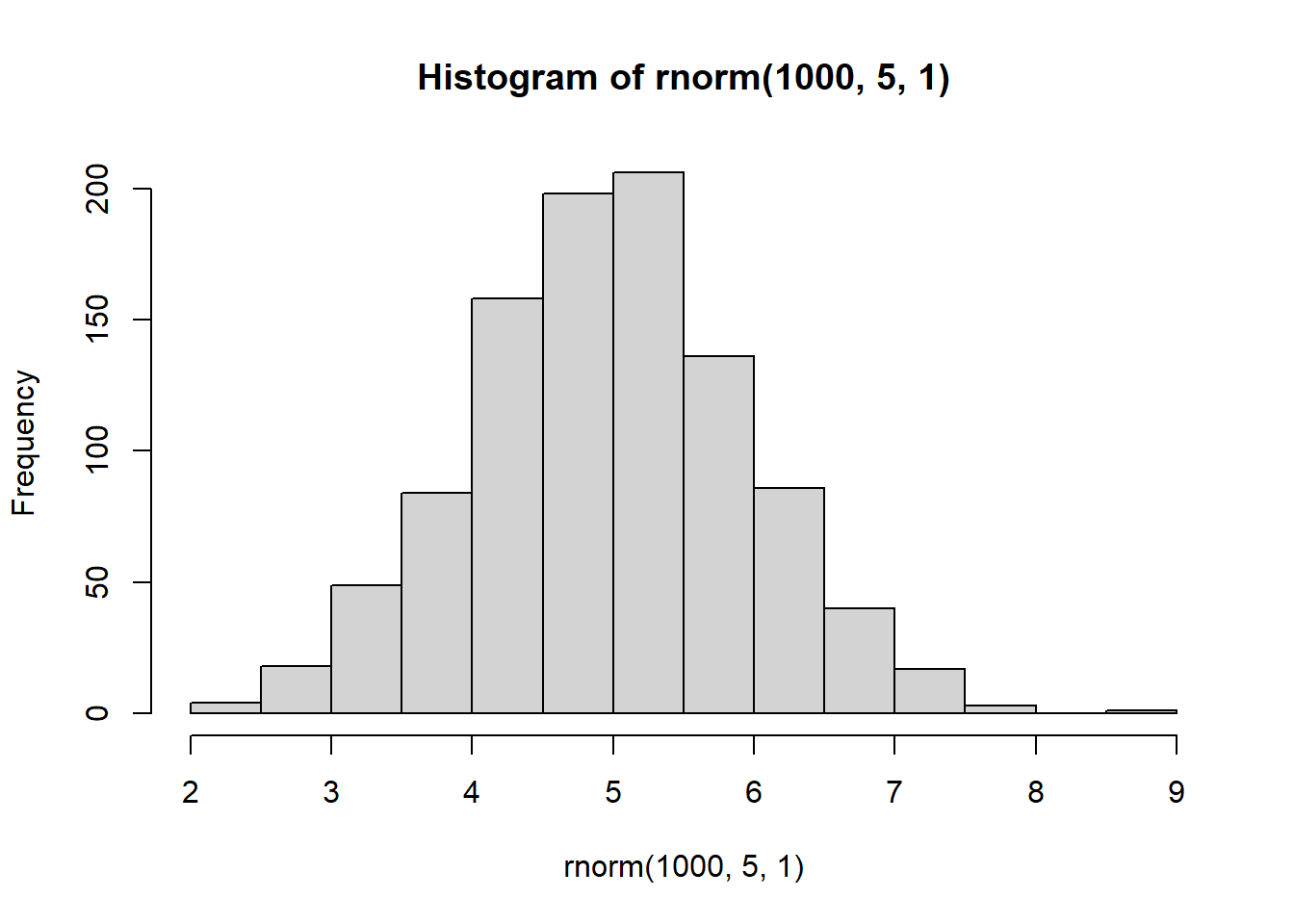

With increasing sample size, the distribution starts to look more normal

We know that in these simulated distributions the mean = 5 and sd = 1.

In theory, with increasing sample size, the estimated mean and SD should get more accurate.

This is because with more data (a larger sample size) we can estimate things more accurately.

mean(rnorm(10,5,1))

[1] 4.825311

mean(rnorm(100,5,1))

[1] 5.027543

mean(rnorm(1000,5,1))

[1] 4.99873

sd(rnorm(10,5,1))

[1] 0.8750469

sd(rnorm(100,5,1))

[1] 1.05303

sd(rnorm(1000,5,1))

[1] 0.9799877

Let’s do something a little more complex…

We are going to use a “loop” - this is a way of performing repeated instructions over a series of iterations (i).

Before we do this, let’s set up our plotting window so that we have a 2 x 2 array of plots.

We must do this first (before plotting):

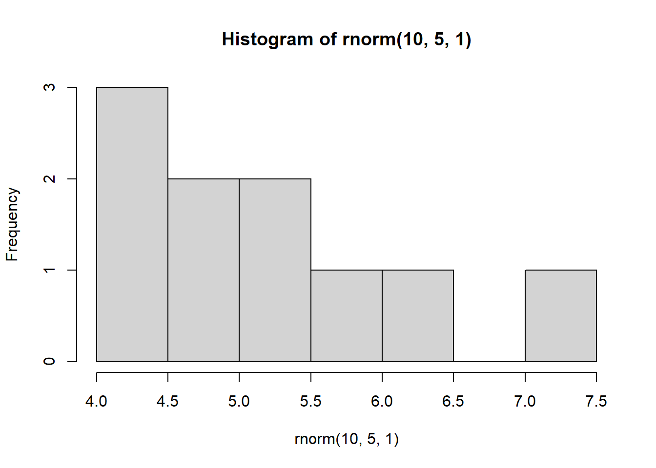
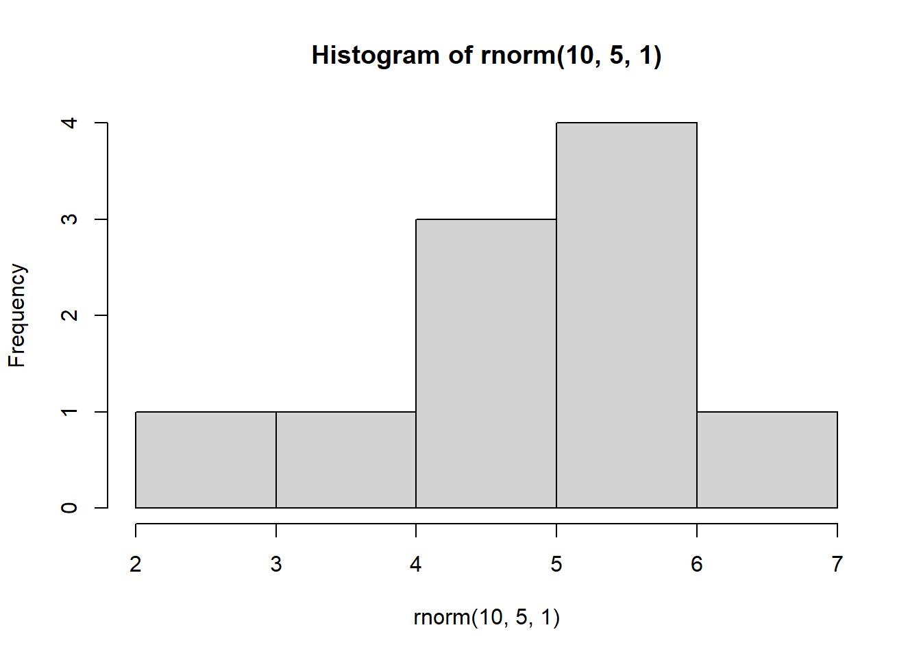
par(mfrow=c(2,2)) # This tells R to plot all subsequent plots in a 2 x 2 array

Now, let’s run a “for loop” to plot 4 histograms, each time with a different sample:

We can interpret this code as follows: For every iteration (i) in iterations 1 to 4, create a histogram of 10 observations drawn from a random normal distribution with a mean = 5 and sd = 1

NOTE: You can run this over and over again, each time it will produce 4 different graphs:

for(i in 1:4) { 
  hist(rnorm(10, 5, 1)) 
  }

Why does this matter?

This demonstrates the impact of replication. Imagine we were to take only a sample of data that consisted of 10 observations. Depending on which 10 observations we happen to select, our sample could look very different!

Often we only perform an experiment once i.e., we only collect the first sample of 10 observations

In fact, we may want to repeat entire experiments multiple times (known as replication) in order to ensure that our results are robust.

Here’s another example of this:

Suppose we were measuring the height of young trees i.e., saplings (cm)

We won’t know in a real experiment what the true population looks like, but usefully in R we can simulate this.

Let’s assume that the population consists of 1000 saplings, and on average they are 50 cm tall, with SD of 5 cm:

saplings <- rnorm(1000, mean = 50, sd = 5)

Let’s imagine now I do an experiment - I sample the heights of just 5 saplings:

saplings1 <- sample(saplings, 5, replace = F)

If I now estimate the mean of that sample, what is it?

mean(saplings1)

[1] 52.47439

Now let’s imagine I repeat that experiment. I go back into the field on a different day and measure 5 saplings again:

saplings2 <- sample(saplings, 5, replace = F)

If I now estimate the mean of that second sample, what is it?

mean(saplings2)

[1] 51.12288

The chances are the means of saplings1 and saplings2 could be quite different to each other and also quite different to the true (simulated) mean of the population

Let’s see what these samples both look like:

Plot to visualize:

par(mfrow=c(1,2))

hist(saplings1, main="Sample 1 (5 saplings)", xlab="Height (cm)", col="lightblue", las = 1)

hist(saplings2, main="Sample 2 (5 saplings)", xlab="Height (cm)", col="lightgreen", las = 1)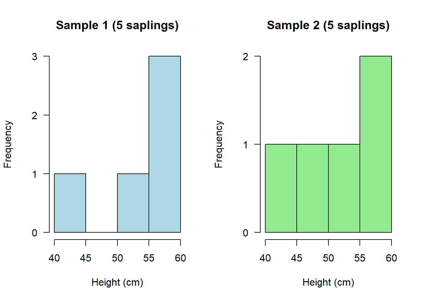

Depending on what you happened to randomly sample on each occasion, these could look quite different!

In other words, when you repeat exactly the same experiment, you might end up with quite different results.

If you were to repeat this experiment many times, then you could calculate an average sapling height across ALL of your experiments. This would be a much more reliable/robust average than if you’d only done the experiment once.

Now let’s have a look at if I were to do the experiment only twice, but this time collect a much larger sample of data on both occasions:

saplings1b <- sample(saplings, 100, replace = F)

saplings2b <- sample(saplings, 100, replace = F)

If we plot them again, we should see that these two distributions now look much more similar:

par(mfrow=c(1,2))

hist(saplings1b, main="Sample 1 (5 saplings)", xlab="Height (cm)", col="lightblue", las = 1)

hist(saplings2b, main="Sample 2 (5 saplings)", xlab="Height (cm)", col="lightgreen", las = 1)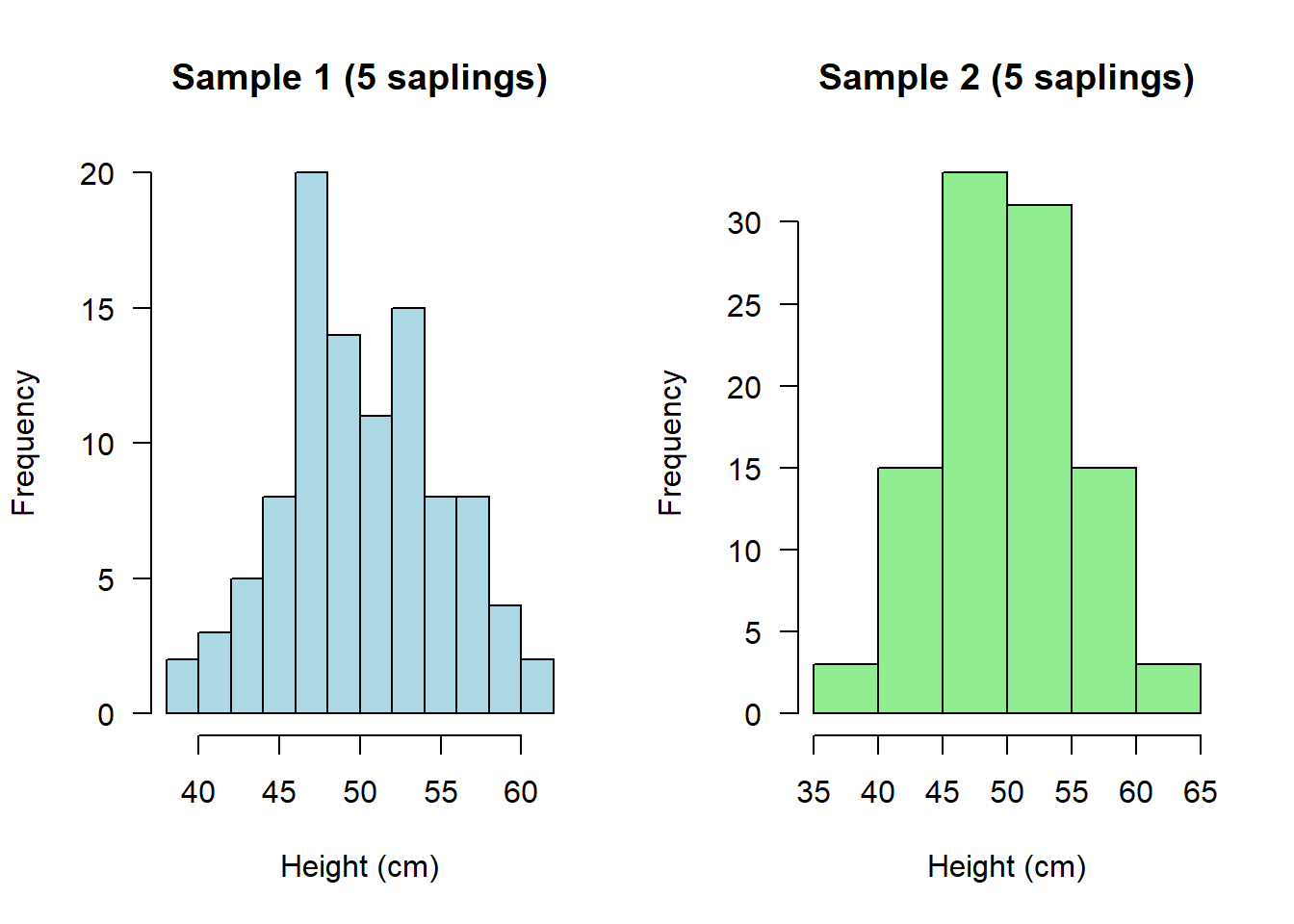

And if we were to calculate their means, not only should these both be more similar to each other, they should also both be more similar to what we know to be the true (simulated) mean in the population:

mean(saplings1b)

[1] 49.99518

mean(saplings2b)

[1] 50.0277

Setting a seed

This may seem like an odd concept, but sometimes we want to generate a random set of numbers that is always the same set of random numbers!

To do this, we set a “seed”. Think of a seed as a specific instance of R.

The seed can be any number and must be set prior to running a random number generator:

set.seed(1); rnorm(5, 5, 1)

[1] 4.373546 5.183643 4.164371 6.595281 5.329508

Notice what I have done on the above line is use the semi-colon “;” - This allows me to run two functions on the same line of code, one after the other.

If you run that line of code above again, you will always get the same 5 random numbers!

Compare that to running the below line of code a few times, without setting a seed. You should get a random set of numbers every time:

rnorm(5, 5, 1)

[1] 4.179532 5.487429 5.738325 5.575781 4.694612

Why is setting a seed useful?

Setting a seed is important for playing with simulations because it ensures results are reproducible every single time. This goes not just for you, but for anyone else running the code.

So, in theory, every single person running the following line of code should get the same set of 5 “random” numbers:

set.seed(1); rnorm(5, 5, 1)

[1] 4.373546 5.183643 4.164371 6.595281 5.329508

Subsetting data

We have already seen some examples of subsetting data from a previous script, but it’s so useful it’s worth seeing a few more examples:

Let’s create a new, simulated dataset.

This time we’re going to create data on Alzheimer’s patients

We are going to do this using a seed so that everyone sees exactly the same simulated data:

set.seed(1); Alzheimers <- data.frame(neurons = c(rnorm(100, 20, 5), rnorm(100, 20, 5)), 
                                      group = rep(c("Asymptomatic","Symptomatic"), each = 100), 
                                      sex = c(rep("M", 50), rep("M", 50), rep("F", 50), rep("F", 50)),
                                      age = round(rnorm(200, 70, 5), 0))

Note that the “neurons” variable represents the neuron cell density in patients

Have a quick look:

head(Alzheimers)

   neurons        group sex age
1 16.86773 Asymptomatic   M  72
2 20.91822 Asymptomatic   M  78
3 15.82186 Asymptomatic   M  78
4 27.97640 Asymptomatic   M  68
5 21.64754 Asymptomatic   M  59
6 15.89766 Asymptomatic   M  82

There are many different ways to subset data:

Selecting for a particular group e.g. Males (all these 4 lines of code achieve the same thing!):

males <- subset(Alzheimers, sex == "M")

males <- subset(Alzheimers, sex %in% "M")

males <- Alzheimers[Alzheimers$sex == "M", ]

males <- Alzheimers[Alzheimers$sex %in% "M", ]

Selecting against a particular group:

Asymptomatic <- subset(Alzheimers, group != "Symptomatic")

Selecting individuals over or under a certain age:

over70 <- subset(Alzheimers, age > 70)

under70 <- subset(Alzheimers, age < 70)

Selecting individuals “greater than or equal to” a certain age:

atLeast60 <- subset(Alzheimers, age >= 60)

Selecting individuals “less than or equal to” a certain age:

age58orLess <- subset(Alzheimers, age <= 58)

Selecting specific rows from a dataset:

first10 <- Alzheimers[1:10,]

last20 <- Alzheimers[181:200,]

Selecting specific rows AND columns:

subset <- Alzheimers[50:100, 1:2] # Select rows 50 to 100, but only data from the first 2 columns

TASKS

Write your own code to complete the following 6 tasks. NOTE: You will not be assessed on these tasks. They are just designed to encourage you to practice.

NOTE: You aren’t expected to remember how to do all of these yet!

HINT: Look back at earlier sections of your script to find the bits of code that you need, and adapt them (that’s the best way to work in R)

Task 1

Write the code to create a randomly generated dataset consisting of observations that follow a Poisson distribution with a mean value of 10. And write the code to plot this distribution.

Task 2

Write the code to execute a loop that plots 4 random poisson distributions where n = 10 and lambda = 2

Task 3

Write the code to subset the Alzheimers data so that you have a sample of 50 random individuals

Task 4

Write the code to plot a histogram of neuron cell density for only Symptomatic Alzheimer’s patients